
How matching probability, waiting costs, and trader participation shape execution decisions.
This explainer uses a small intent-auction model from the earlier CoW welfare research. Its values are normalized model units, not production CoW measurements.
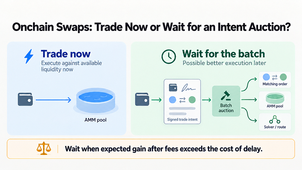
Fig. 1. A trader can execute immediately against available liquidity or wait while Solvers search for better execution through matching orders and external liquidity routes, including AMMs.
Would you wait for a better price?
Suppose an immediate AMM swap is available now. Waiting might improve execution by 10 dollars with a 30% chance, but costs 1 dollar in fees and 1.50 dollars in delay risk. Expected net gain, in dollars: 10 × 0.30 − 1 − 1.50 = +0.50. At an 18% chance it is −0.70.
The break-even probability is 25%: (1 + 1.50) / 10. Below it, waiting loses money. In this simplified example, the auction order is assumed to execute even without a price improvement. The fee is an incremental cost relative to trading immediately. An unfilled CoW order, however, does not incur an execution fee. These dollars are illustrative, not a CoW quote.
How does the model see this choice?
The 10-dollar example takes the 30% chance as given; the model asks where it comes from. In a batch auction, a better match depends on how many other traders wait. This is the thick-market idea from matching theory (Diamond, 1982; Roth, 2008): each trader improves the market for others but decides on their own gain and delay cost.
The same mechanism, fee, and batch length can sustain itself in one market and empty out in another. If enough traders wait, matches become likely and waiting keeps paying; if too few wait, the chance falls, more traders leave, and it falls further. A single quote cannot show which side of that line a market is on.
In this model, q represents the probability of realizing the assumed execution gain. It does not separately identify direct order matching and improvements obtained through external liquidity. Only direct matching grows with the number of traders waiting; a better route through AMMs or market makers does not, and the model treats both as one chance of a better match to keep the feedback loop simple.
Two equations capture this loop. The first gives the chance of a match when a share Vₜ of traders is waiting:
The second gives the share that waits next. A trader waits when the expected gain after the fee covers their own delay cost, aq − f ≥ wᵢΔ/2; with waiting costs spread uniformly from zero to w̄,
Key parameters.
q₀ — baseline chance of a match before any extra waiting.Vₜ — share of traders waiting in the batch at step t.Δ — batch duration; the expected wait is Δ/2.e — Solver effort; with λ₀ and β, it sets how fast new matching opportunities arrive.a — trader’s gain when a better match arrives.f — fee paid for waiting, whether or not the match improves (a modelling simplification; CoW charges fees only when an order executes).w̄ — upper end of individual waiting costs.
In plain English. A match might be an opposite ETH/USDC intent, avoiding AMM fees, or a Solver finding a better route across AMMs, aggregators, or a market maker. Waiting creates another chance; it improves with participation, Solver effort, or batch length.
Only traders for whom that chance pays for delay stay in the batch, setting the next matching chance. With 20% waiting and q₀ = 0.25, it is 27.7% and about 32% wait next. With q₀ = 0.18, it is 21.0% and only about 4% wait.
What does waiting buy?
Hold participation fixed and stretch the batch. Matching chance rises, but each extra increment buys less than the last.
Fig. 2. This figure isolates matching technology at q₀ = 0.25, with full participation and fixed Solver effort. A 38% chance among 100 participating orders means about 38 expected orders realizing the modeled improvement, rather than 38 guaranteed bilateral pairs.
Delay cost grows with the wait, so a longer batch eventually stops paying. Fig. 2 assumes everyone waits; with 20 of 100 waiting, the same batch gives 27.7%, not 37.7%.
Why do other traders matter?
Fig. 3 runs the loop above from the same starting point in two markets that differ only in q₀.
Fig. 3. Both cases begin with 20 of 100 potential traders. The figure shows a fixed-effort participation update: a decision mapping rather than a block-by-block market history.
At q₀ = 0.25, 20 participants become about 32, then settle near 47. At q₀ = 0.18, they become about four, then zero as departures lower the remaining chance.
These paths illustrate participation feedback under fixed Solver effort, rather than observed market dynamics or equilibria of the full Solver-Trader game.
Does a better match create value?
A better execution makes the trader privately better off. It does not establish that the market saved resources rather than reassigned a payment.
This comparison uses w̄ = 8, V = 1, Δ = 0.20, winning Solver effort 0.40, and no effort from the other Solver. Waiting costs 0.400; the winner’s effort costs 0.6 × 0.40² = 0.096 (c = 1.20), and fixed operating cost is O = 0.02, totaling 0.516.
Both cases give five units of private improvement per successful match. In the transfer-heavy case, four are another participant’s foregone income and one is a real saving; in the resource-heavy case, the split is one transfer and four real savings. With every trader waiting (V = 1), the matching chance is q = 0.377, the 38% point in Fig. 2. Real saving per trader is then 1 × 0.377 − 0.516 = −0.139 in the transfer-heavy case and 4 × 0.377 − 0.516 ≈ +0.993 in the resource-heavy case.
How does this translate to a real trade?
Before waiting, ask three things: how large might the improvement be, what is the chance of receiving it, and what does delay cost? A quote tells you what you could receive under specified conditions. It does not tell you the chance of a better quote after waiting.
Real CoW batches are richer than this toy market: Solvers draw on other orders, AMMs, aggregators, and private market makers, and an order can stay open across several auctions (CoW documentation). The values 0.25 and 0.18 are illustrations, not observed CoW market states.
Waiting pays only when the expected execution improvement exceeds its incremental costs. Even then, a better trade for the individual does not necessarily mean greater welfare for the market.
Appendix
Parameter values. Matching: q₀ ∈ {0.25, 0.18}, λ₀ = 0.45, β = 1.2, e = 0.40. Participation: a = 5, f = 1, w̄ = 12, Δ = 0.20, starting from V = 0.20. Welfare uses its own setting (w̄ = 8, V = 1). Figures in the text are rounded; calculations are not.Model and figures. Executable notebook.Background. Diamond, P. A. (1982). Aggregate demand management in search equilibrium. Journal of Political Economy, 90(5), 881–894. Roth, A. E. (2008). What have we learned from market design? Economic Journal, 118(527), 285–310.Related. Execution surplus and welfare in a simplified intent-auction game.
This post was originally published on my personal blog: https://egpivo.dev/articles/when-does-waiting-for-a-better-trade-pay-off.
Onchain Swaps: Trade Now or Wait for an Intent Auction? was originally published in Coinmonks on Medium, where people are continuing the conversation by highlighting and responding to this story.