How zkSNARKs Actually Work: R1CS, QAP, and Pairings Explained With Examples

2. Zero Knowledge From Mental Model to Math: What Actually Happens Inside a zkSNARK

Part 2 of a 4-part series. In Part 1, we built the mental model. In Part 3, we’ll cover zero-knowledge and Groth16. Part 4 re-implements TornadoCash.

I know this post is a little bit long, but trust me it’s better to have all the math in one place rather than trying to figure out what is happening in several posts.

In the previous post we built the intuition. A prover convinces a verifier that they know something, without revealing what they know.

Now let’s open the hood.

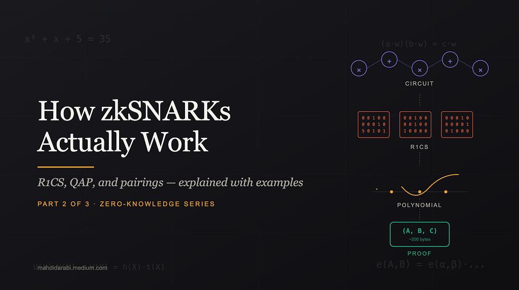
How does a piece of code, like x³ + x + 5 = 35, become a cryptographic proof that is only 200 bytes and takes about 1 millisecond to verify?

That’s not metaphor. That’s what zkSNARKs actually deliver.

To get there, we’ll walk through four big ideas:

Turning computation into gatesTurning gates into constraints (R1CS)Turning constraints into a single polynomial equation (QAP)Using elliptic curve pairings to check that equation without revealing anything

No magic. Just careful layering. And at every step, real numbers you can verify yourself (I strongly suggest to the math by yourself, so it’s better to bring pen and paper).

Let’s start.

The Example We’ll Carry Through the Whole Post

We want to prove:

“I know a value x such that x³ + x + 5 = 35”

Without revealing x.

Spoiler: x = 3. But the prover will never say that. The verifier will just get a 200-byte proof, and a “yes, they know it.”

This is a tiny toy. Real zkSNARKs prove things like “I performed a valid Zcash transaction” or “this ML model was evaluated correctly.” But the machinery is identical. If you understand x³ + x + 5, you can understand Zcash.

Step 1: Turning Computation Into Gates

A computer doesn’t “know” algebra. It knows how to add, and how to multiply. Everything else is built on top.

So the first step of any zkSNARK is to flatten the computation into a sequence of very simple statements — each one either an addition or a multiplication.

The Flattening Rule

Every statement must look like:

variable = variable (op) variable

Where op is +, -, *, or /. And each operation takes exactly two inputs.

No nested expressions. No “do three things at once.” Just one operation per line.

Why This Restriction?

Three reasons, each important:

1. It matches how real CPUs work. An ADD r1, r2, r3 instruction means “add r2 to r3, store in r1.” Flattening is essentially the assembly-language trace of your program.

2. Every intermediate value gets named. If your computation has unnamed sub-expressions, you can’t pin them down cryptographically. By naming every intermediate, we create variables the prover must commit to.

3. It maps cleanly to the next step. Each multiplication gate will become exactly one row of R1CS. If we allowed 3-input gates, that clean 1-to-1 mapping would break.

Flattening Our Example

The expression x³ + x + 5 isn’t atomic. Let’s break it down:

sym_1 = x * x ← computes x²
sym_2 = sym_1 * x ← computes x³
out = (sym_2 + x + 5) * 1 ← the final sum

Three lines. Each one a single gate.

Every intermediate value gets its own name (sym_1, sym_2). These names matter — they become witness variables later.

The Circuit View

Picture this as a circuit — a network of gates wired together:

x³ + x + 5 to gates of addition and multiplication

Each gate has two inputs — Left and Right — and one output. The output of one gate can fan out to become the input of many later gates. This shape — gates wired by their inputs and outputs — is the foundation of everything that follows.

Free vs. Expensive Operations

Here’s a practical fact that shapes how real ZK circuits are designed:

Operation Cost a + b free a − b free 5 × a (times a constant) free a + 7 (plus a constant) free a × b (between two secrets) 1 constraint a × a (squaring) 1 constraint

Only multiplications between two secret variables cost something (and thus a constraint).

This is why ZK-friendly hash functions like Poseidon exist. A SHA-256 invocation takes roughly 27,000 multiplication constraints. Poseidon hashes the same amount of data in around 200 constraints — over 100× cheaper. When you hear “this circuit has 30,000 constraints,” they always mean 30,000 multiplication gates.

Step 2: Constraints With Three Slots (L · R = O)

Now here’s the cleanest idea in the whole system.

Every multiplication gate becomes one constraint with three slots:

(Left input) × (Right input) = (Output)

We call this R1CS — Rank-1 Constraint System. The “rank 1” means each constraint is one linear thing times one linear thing equals one linear thing.

Each Slot Is a Linear Combination

This is the twist that makes R1CS powerful. Each slot doesn’t have to be just one variable. It can be a sum of variables, each multiplied by some coefficient.

For example, a valid R1CS constraint could look like:

(2x + 3y + 5) × (z) = (out)

The left slot is a linear combo. The right slot is just z. The output is just out. Still one constraint.

Why allow this? Because additions are free. If your circuit needs to sum several numbers before multiplying, we pack those additions directly into the slot. No extra gates. No extra constraints.

Think of each slot as a little “pre-processor” that can take as many witness values as it wants, weight them, sum them up — and hand the result to the multiplication.

The Witness Vector

To express these linear combinations, we put all the variables into one ordered list called the witness.

For our example:

w = (1, out, x, sym_1, sym_2)

By convention:

Position 0 is always 1 (the constant wire — this lets us inject constants like 5 into linear combinations)Then the public variables (like out)Then the private variables and intermediates (x, sym_1, sym_2)

With x = 3:

w = (1, 35, 3, 9, 27)

This is the complete witness. The prover knows all 5 values. The verifier knows only the public part: w[0] = 1 and w[1] = out = 35.

Anatomy of One Constraint

Here’s the shape in full detail:

(a₀·w₀ + a₁·w₁ + a₂·w₂ + …) ×
(b₀·w₀ + b₁·w₁ + b₂·w₂ + …) =
(c₀·w₀ + c₁·w₁ + c₂·w₂ + …)

The coefficients (a₀, a₁, …, b₀, b₁, …, c₀, c₁, …) are fixed at circuit design time. They’re part of the public description of the problem. The prover doesn’t choose them.

What the prover does choose is the witness w.

Think of each constraint as a stencil: three patterns that, when laid over the witness, extract three numbers. The constraint is “those three numbers must satisfy L × R = O.”

How gate3 works in Left, Right, Output system

Writing Each Gate as a Constraint

Let’s do all three gates of our example. This is where you should slow down and trace with pen and paper — the pattern is simple once you see it.

costly operators are blue, and free operators are green

Gate 1: x × x = sym_1

Left slot picks x: a = (0, 0, 1, 0, 0)Right slot picks x: b = (0, 0, 1, 0, 0)Output slot picks sym_1: c = (0, 0, 0, 1, 0)

Verify:

a · w = 0 + 0 + 1·3 + 0 + 0 = 3b · w = 3c · w = 0 + 0 + 0 + 1·9 + 0 = 9Check: 3 × 3 = 9 ✓

Notice a and b are identical here. That’s how we encode squaring — plug the same variable into both ports.

Gate 2: sym_1 × x = sym_2

a = (0, 0, 0, 1, 0) → picks sym_1b = (0, 0, 1, 0, 0) → picks xc = (0, 0, 0, 0, 1) → picks sym_2

Verify:

a · w = 9b · w = 3c · w = 27Check: 9 × 3 = 27 ✓

Here the output of gate 1 (sym_1 = w[3] = 9) becomes the left input of gate 2. In R1CS this is just “select w[3] in the Left slot” — simple.

Gate 3: (sym_2 + x + 5) × 1 = out

How gate3 works in Left, Right, Output system

This gate shows off linear combinations. The left side is three things added together.

Left slot: 5·w[0] + 1·w[2] + 1·w[4], so a = (5, 0, 1, 0, 1)Right slot: just 1, so b = (1, 0, 0, 0, 0)Output slot: just out, so c = (0, 1, 0, 0, 0)

Verify:

a · w = 5·1 + 1·3 + 1·27 = 35 ← the sum (sym_2 + x + 5)b · w = 1c · w = 35Check: 35 × 1 = 35 ✓

This gate uses three R1CS tricks at once:

Constant injection via w[0] = 1: the coefficient 5 on position 0 means “add the constant 5 to this slot”Multi-wire linear combination: three variables (w[0], w[2], w[4]) contribute to one slotMultiply by 1: since gate 3 is really just addition, we multiply by 1 to fit the L·R=O shape

Here’s what all three gates look like laid out together:

Stacking Into Matrices

Now we collect all the a vectors into a matrix A, all the b vectors into B, all the c vectors into C. Each row is one gate:

w₀ w₁ w₂ w₃ w₄ w₀ w₁ w₂ w₃ w₄ w₀ w₁ w₂ w₃ w₄
┌ ┐ ┌ ┐ ┌ ┐
A = │ 0 0 1 0 0│ B = │ 0 0 1 0 0│ C = │ 0 0 0 1 0│
│ 0 0 0 1 0│ │ 0 0 1 0 0│ │ 0 0 0 0 1│
│ 5 0 1 0 1│ │ 1 0 0 0 0│ │ 0 1 0 0 0│
└ ┘ └ ┘ └ ┘

The R1CS condition is:

(A·w) ⊙ (B·w) = C·w

where ⊙ is componentwise multiplication. All three constraints collapsed into one matrix equation.

Let me verify:

A·w = (3, 9, 35)B·w = (3, 3, 1)Componentwise product: (9, 27, 35)C·w = (9, 27, 35) ✓

All three constraints hold. The witness is valid.

Two Ways to Read These Matrices

Row-wise: Each row is one gate’s stencil. This is how you check a witness.

Column-wise: Each column is one variable’s “participation pattern across gates.” Column 2 (index 2 actually, column 3) of A says: “variable x shows up in the Left slot of gate 1 (coefficient 1), not in gate 2 (coefficient 0), and in gate 3 (coefficient 1).”

This column view is the key conceptual shift for the next step. We’re about to turn each column into a polynomial.

Step 3: One Polynomial to Rule Them All

We now have 3 constraints (We are talking about each column of each matrix, A, B or C). Checking 3 constraints is no problem. But real ZK circuits have millions of constraints. Checking them one by one isn’t succinct — it’s not even close.

We need to collapse all constraints into one equation.

The tool: polynomial interpolation.

The Core Idea

Pick 3 distinct points — say x = 1, 2, 3. Think of each point as “the index of one gate (constraint actually).”

(Again we are talking about each column of each matrix, now matrix A)

For each witness variable j, we build a polynomial that encodes its participation in the L slot across all gates:

u_j(1) = coefficient of w_j in gate 1’s L slot
u_j(2) = coefficient of w_j in gate 2’s L slot
u_j(3) = coefficient of w_j in gate 3’s L slot

Three points, one polynomial. Lagrange interpolation gives us a unique polynomial of degree ≤ 2 through any 3 points.

for example, we now Talking about matrix A and column with index 2 (third column).

matrix Au_2(1) = 1
u_2(2) = 0
u_2(3) = 1

We do the same for the R slot (getting v_j polynomials) and the O slot (getting w_j polynomials — warning, overloaded notation: w_j the polynomial is different from w[j] the witness value).

Building a Polynomial from Scratch — Worked Example

Let’s build u_x(λ) for our variable x (index 2 in the witness).

Looking at column 2 of matrix A, x appears with coefficients:

Gate 1 Left: 1Gate 2 Left: 0Gate 3 Left: 1

So we want a polynomial u_x(λ) (or it’s better to write u_2(λ) because “x” is index 2 of witness array) with:

u_2(1) = 1u_2(2) = 0u_2(3) = 1

Lagrange interpolation gives us a recipe. For 3 points (1, 2, 3), the basis polynomials are:

ℓ₁(λ) = (λ − 2)(λ − 3) / 2
ℓ₂(λ) = −(λ − 1)(λ − 3)
ℓ₃(λ) = (λ − 1)(λ − 2) / 2

Each ℓᵢ equals 1 at its own point and 0 at the other two. So:

u_2(λ) = 1·ℓ₁(λ) + 0·ℓ₂(λ) + 1·ℓ₃(λ)
= (λ−2)(λ−3)/2 + (λ−1)(λ−2)/2
= (λ−2)·[(λ−3) + (λ−1)] / 2
= (λ−2)(2λ−4)/2
= (λ−2)²
= λ² − 4λ + 4u_2(λ) = λ² -4λ + 4

Check:

u_2(1) = 1 − 4 + 4 = 1 ✓u_2(2) = 4 − 8 + 4 = 0 ✓u_2(3) = 9 − 12 + 4 = 1 ✓

This is the polynomial encoding “how x (index 2 of witness) participates in the Left slot across our three gates.”

We do this for every witness variable, for all three slot types (L, R, O). That gives us a whole library of polynomials. They’re all computed from the circuit, once — not per-witness.

The Combined Polynomials

Once we have all the per-variable polynomials, we build three big polynomials by summing them weighted by the witness:

U(λ) = sum over all j of (w[j] · u_j(λ)) ← the combined Left
V(λ) = sum over all j of (w[j] · v_j(λ)) ← the combined Right
W(λ) = sum over all j of (w[j] · w_j(λ)) ← the combined Output

The magic property:

U(i) = the Left slot value of gate i
V(i) = the Right slot value of gate i
W(i) = the Output slot value of gate i

(Do not cofuse above “W” with witness)

(for i = 1, 2, 3 — the three gate indices)

For our witness w = (1, 35, 3, 9, 27), a bit of arithmetic gives:

U(λ) = 10λ² − 24λ + 17V(λ) = −λ² + 3λ + 1W(λ) = −5λ² + 33λ − 19

Verify U, V, W at Every Gate Index

This is where you can see the construction really works. Plug in λ= 1, 2, 3:

At λ= 1 (gate 1):

U(1) = 10 − 24 + 17 = 3 (Left of gate 1 = x = 3 ✓)V(1) = −1 + 3 + 1 = 3 (Right of gate 1 = x = 3 ✓)W(1) = −5 + 33 − 19 = 9 (Output of gate 1 = sym_1 = 9 ✓)

At λ= 2 (gate 2):

U(2) = 40 − 48 + 17 = 9 (Left of gate 2 = sym_1 = 9 ✓)V(2) = −4 + 6 + 1 = 3 (Right of gate 2 = x = 3 ✓)W(2) = −20 + 66 − 19 = 27 (Output of gate 2 = sym_2 = 27 ✓)

At λ= 3 (gate 3):

U(3) = 90 − 72 + 17 = 35 (Left of gate 3 = sym_2 + x + 5 = 35 ✓)V(3) = −9 + 9 + 1 = 1 (Right of gate 3 = 1 ✓)W(3) = −45 + 99 − 19 = 35 (Output of gate 3 = out = 35 ✓)

The polynomials literally encode the gate computations. Every gate’s constraint becomes:

U(i) × V(i) − W(i) = 0

The Key Identity

Define the polynomial:

P(λ) = U(λ) · V(λ) − W(λ)

From the checks above:

P(1) = 3·3 − 9 = 0P(2) = 9·3 − 27 = 0P(3) = 35·1 − 35 = 0

P(λ) vanishes at λ= 1, 2, 3. Which means P(λ) is divisible by:

t(λ) = (λ − 1)(λ − 2)(λ − 3)

t(λ) is called the target polynomial. It’s a public property of the circuit — once the circuit is fixed, t(λ) is fixed too.

And the quotient:

h(λ) = P(λ) / t(λ)

is a clean polynomial with no remainder — but only if all constraints are satisfied.

If even one constraint fails, P(λ) won’t vanish at the corresponding gate index, and t(λ) won’t divide P(λ) cleanly.

The QAP: One Equation for Everything

So the entire R1CS collapses into this one equation:

U(λ) · V(λ) − W(λ) = h(λ) · t(λ)

This is a QAP — Quadratic Arithmetic Program. One equation. Any number of gates.

A Sanity Check at a Random Point

Let me show you that this is a real polynomial identity, not a coincidence at the three gate points.

At λ= 5:

U(5) = 250 − 120 + 17 = 147V(5) = −25 + 15 + 1 = −9W(5) = −125 + 165 − 19 = 21P(5) = 147·(−9) − 21 = −1323 − 21 = −1344

Now t(5) = 4·3·2 = 24. And you can compute h(λ) = −10λ − 6 (it’s linear because h has degree 4 − 3 = 1), so h(5) = −56.

h(5) · t(5) = −56 · 24 = −1344 ✓

Match. The identity holds everywhere — not just at the gate points — because it’s a real polynomial equation.

Why This Matters

We’ve moved from “check 3 constraints” to “check whether one polynomial divides another.”

For a 30-million-gate circuit, this is a massive win: instead of 30 million separate checks, we have one polynomial identity that captures all of them.

But we still have one problem: how do we check this identity without revealing the witness?

That’s the last piece — elliptic curves and pairings.

Step 4: Elliptic Curve Pairings — Checking Without Seeing

We now need a way for the prover to commit to values like U(τ), V(τ), W(τ), h(τ), and let the verifier check the polynomial identity — without anyone ever learning what these values are.

This is where elliptic curves come in.

The Basic Tool: Scalar Multiplication on a Curve

you need to know a little bit about Elliptic curve, unless you can not follow what’s happening. Mastering Bitcoin is a good source to understand what’s the concept of Elliptic curves

An elliptic curve gives us a special group. I won’t go deep into the math, but the key facts are:

You have a generator point G“Multiplying” G by a scalar a means adding G to itself a times: [a]G = G + G + … + GComputing [a]G from a is easyComputing a from [a]G is cryptographically hard — this is the discrete log problem (the fundamental security for public key private key signatures)

So [a]G is a one-way commitment to a. You can share it without revealing a.

And importantly, these commitments preserve addition:

[a]G + [b]G = [a + b]G

So if I’ve committed to a and b, I can get a commitment to a + b for free.

The Problem: We Need Multiplication, Not Just Addition

The QAP identity involves U(τ) × V(τ). That’s a multiplication in the exponent. And plain elliptic curves don’t let us multiply commitments.

If I give you [a]G and [b]G, you cannot compute [a·b]G efficiently. That would break discrete log.

So how do we check a multiplicative relationship?

u·v — w ?= ht

Enter Pairings

A pairing is a special function between three groups:

e: G₁ × G₂ → G_T

with one magical property — bilinearity:

e([a]G₁, [b]G₂) = e(G₁, G₂)^(a·b)

In words: feed the pairing two committed values, and it gives you a value where the product a·b sits in the exponent (of a third group).

This is exactly what we need.

Using Pairings to Check Multiplication

Suppose the prover gives the verifier [u]₁

a commitment to U(τ) in group G₁like [U(τ)]Generaror1 which is the scalar multiplication of U(τ) in Generator point of group G1this format applies for the next commitments like [v]₂ etc.

and [v]₂ (a commitment to V(τ) in group G₂).

The verifier computes e([u]₁, [v]₂), which equals e(G₁, G₂)^(u·v). Call this value LHS.

Separately, suppose the prover gives [w]₁ (commitment to W(τ) in Group G1) and [ht]₁ (commitment to h(τ)·t(τ) in Group G1).

The verifier computes e([w]₁ + [ht]₁, G₂) = e(G₁, G₂)^(w + ht). Call this RHS.

If LHS == RHS, then u·v = w + ht in the exponent. Which means the QAP identity holds at τ.

The verifier learned nothing beyond the fact that the equation balanced. No witness values, no polynomial coefficients. Just a yes/no answer.

The Trusted Setup: Where Does τ Come From?

One problem: how does the prover compute commitments at τ when τ is secret?

Setup ceremony: A trusted party (or a multi-party computation) samples τ randomly. Then they publish:

[1]₁, [τ]₁, [τ²]₁, [τ³]₁, … (up to the degree needed)

And analogously in G₂.

This collection is called the Structured Reference String (SRS).

Then τ is destroyed. Nobody should ever know it.

Why Destroying τ Matters

If τ leaked, a cheater could:

Compute t(τ) directlyFind polynomials U’, V’, W’, h’ that satisfy U’(τ)·V’(τ) − W’(τ) = h’(τ)·t(τ) at that specific τ but correspond to no real witnessForge a valid-looking proof

This is called the toxic waste problem. Real ceremonies are elaborate. The Zcash Sapling ceremony used dozens of participants, each contributing randomness. Only one participant needs to be honest and destroy their share for the setup to be safe.

Committing to a Polynomial Without Knowing τ

Here’s the beautiful part: even though the prover doesn’t know τ, they can still commit to any polynomial f(X) at τ.

If f(X) = c₀ + c₁·X + c₂·X² + c₃·X³, then the prover computes:

[f(τ)]₁ = c₀·[1]₁ + c₁·[τ]₁ + c₂·[τ²]₁ + c₃·[τ³]₁

This is a linear combination of SRS elements — no τ knowledge required. The result is a single group element encoding f(τ) in the exponent.

The prover’s coefficients c₀, c₁, … come from the witness via the column polynomial construction from Step 3.

Schwartz-Zippel: Why Checking at One Point Is Enough

There’s a subtle worry. The verifier only checks the QAP identity at one point (τ). How do they know the identity truly holds as polynomials — not just at that one lucky point?

Schwartz-Zippel lemma: If two polynomials of degree ≤ d are different, they disagree at almost every point. Specifically, they agree at most at d points out of the whole field.

So if a cheating prover tries to make the identity hold at τ without actually being a real polynomial identity, their success probability is at most d/p, where p is the field size.

With “p” is about (2²⁵⁴) and “d” around 10⁶ for real circuits, this is about 2⁻²³⁴. Essentially zero.

One random check is enough. That’s the miracle that makes zkSNARKs succinct.

Putting It All Together

Here’s the entire pipeline, end to end:

Every modern zkSNARK — Groth16, PLONK, Marlin — follows some version of this pipeline. The details differ (different arithmetizations, different commitment schemes, different setup requirements), but the skeleton is the same.

What We’ve Covered

Let’s take a breath and zoom out.

You’ve now seen the entire machinery that makes zkSNARKs succinct — small proofs, fast verification, for arbitrarily large computations:

Code → Circuit: flatten computation into addition and multiplication gatesCircuit → R1CS: each multiplication gate becomes one constraint with L · R = O shapeR1CS → QAP: interpolate all constraints into one polynomial identityQAP → Pairings: check the identity at a secret point τ using elliptic curve pairings, without revealing anything

Four translations. Each one compressing the computation a little further. Ending in a 200-byte proof that verifies in milliseconds.

But We’re Not Done Yet

Here’s the thing. Everything we built so far makes the proof succinct. But there’s one property we promised and haven’t delivered: zero-knowledge.

Think about it. If the prover commits to U(τ), V(τ), W(τ), h(τ) and the verifier checks the pairing equation, the proof is succinct — but it’s also deterministic. Run the prover twice on the same witness, get the same proof.

That’s a problem. A verifier who guesses the witness could just run the prover themselves and compare. If the proofs match, their guess was right. Information about the witness leaks through the proof’s fingerprint.

So we need one more layer. We need the proof to look uniformly random — to truly reveal nothing beyond “the statement is true.”

What’s Next

In the next post, we’ll finish the job. We’ll see:

Blinding: how random noise gets mixed into the commitments to scramble every proofThe simulator argument: how zero-knowledge is formally proven, not just assertedGroth16 specifics: the four secrets (α, β, γ, δ) and the distinct attack each one defends againstThe trusted setup ceremony: toxic waste, multi-party computation, and destroyed laptopsReal-world numbers: Zcash, TornadoCash, zkEVMs — how all this machinery performs in production

If this post gave you the succinctness of zkSNARKs, the next one gives you the zero-knowledge — the other half of the name, and arguably the more beautiful half.

Then in Part 4, we’ll take everything and re-implement TornadoCash from scratch.

Until then — homework suggestion: pick a different tiny circuit, like (x + 2) × (y + 3) = 21, and do the entire flattening → R1CS → QAP pipeline by hand. Find the witness. Build U, V, W. Check that UV − W vanishes at the gate points.

It’s the best way to lock in what you’ve learned. Once you’ve watched the polynomials cancel with your own pen, this stops being abstract and becomes something you own.

If you enjoyed this, hit 👏 and follow. Part 3 on zero-knowledge is coming soon.

How zkSNARKs Actually Work: R1CS, QAP, and Pairings Explained With Examples was originally published in Coinmonks on Medium, where people are continuing the conversation by highlighting and responding to this story.